5.13. Change of basis sets

Although the computational basis (\(z\)-basis) \(\{|0\rangle,|1\rangle\}\) is the primary basis set, in some cases \(x\)-basis \(\{|+\rangle,|-\rangle\}\) and \(y\)-basis \(\{|L\rangle,|R\rangle\}\) are more convenient.

We can change from a basis set to another by \(H\), \(S\), and \(S\cdot H\).

\[\begin{split} \begin{align} H |0\rangle &= |+\rangle, & \quad H|1\rangle &= |-\rangle \\ S |+\rangle &= |L\rangle, &\quad S|-\rangle &= |R\rangle \\ (S\cdot H)|0\rangle &= |L\rangle, \quad & (S\cdot H)|1\rangle &= |R\rangle \end{align} \end{split}\]

and their inverse transformation are

\[\begin{split} \begin{align} H |+\rangle &= |0\rangle, & \quad H|-\rangle &= |1\rangle \\ S^\dagger |L\rangle &= |+\rangle, &\quad S^\dagger|R\rangle &= |-\rangle \\ (H\cdot S^\dagger)|L\rangle &= |0\rangle, \quad & (H\cdot S^\dagger)|R\rangle &= |1\rangle \end{align} \end{split}\]

5.13.1. Transformation of gates

Consider the following three transofrmations by gates, \(G_z\), \(G_x%\), and \(G_y\).

\[\begin{split} \begin{eqnarray} G_z \left (a_0 |0\rangle + a_1 |1\rangle\right) &=& b_0 |0\rangle + b_1 |1\rangle \\ G_x \left (a_0 |+\rangle + a_1 |-\rangle\right) &=& b_0 |+\rangle + b_1 |-\rangle\\ G_y \left (a_0 |L\rangle + a_1 |R\rangle\right) &=& b_0 |L\rangle + b_1 |R\rangle \end{eqnarray} \end{split}\]

The difference is only the basis set and the coefficients are the same in all three cases. Then, there are simple relation among the gates.

\[ G_z = H \cdot G_x \cdot H, \quad G_y = S \cdot G_x \cdot S^\dagger = (S \cdot H) \cdot G_z \cdot(H \cdot S^\dagger) \]

Example 1 Swapping coefficients

Suppose that a state vector is given in \(\{|+\rangle,|-\rangle\}\) basis as \(c_0 |+\rangle + c_1 |-\rangle\). We want to swap the coefficients.

\[ c_0 |+\rangle + c_1 |-\rangle \quad \xrightarrow{?} \quad c_1 |+\rangle + c_0 |-\rangle \]

What gate do we need? In Section 5.6, we learned that XGate swaps the coeeficients in the computational basis. Recalling that HGate switches basis set between the computational basis and the \(x\)-basis. Then, \(H \cdot X \cdot H\) should do the job. Let us try it.

\[ c_0 |+\rangle + c_1 |-\rangle \quad \xrightarrow{H} \quad c_0 |0\rangle + c_1 |1\rangle \quad \xrightarrow{X} \quad c_1 |0\rangle + c_0 |1\rangle \quad \xrightarrow{H} \quad c_1 |+\rangle + c_0 |-\rangle \]

REcall that we derived \(Z=H \cdot X \cdot H\) in Section 5.9. \(Z\) is the gate we wanted.

---

Exercise 5.13.1  We want to swap the coefficients in the \(y\)-basis. That is \( c_0 |L\rangle + c_1 |R\rangle \quad \xrightarrow{?} \quad c_1 |L\rangle + c_0 |R\rangle \). Find an gate for this transformation.

Exercise 5.13.2  In Section 5.10, we noticed that \(S\) gate and \(SX\) gate work in the same way but in different basis sets. Show that \(SX = H \cdot S \cdot H\) and \(SX^\dagger = H \cdot S^\dagger \cdot H\).

---

Example 2 addition and subtraction of the coefficients

We want to find a gate that transforms a state vector as

\[ c_0 |+\rangle + c_1|-\rangle \quad \xrightarrow{?} \quad \frac{1}{\sqrt{2}}\left(c_0+c_1\right)|+\rangle + \frac{1}{\sqrt{2}}\left(c_0-c_1\right)|-\rangle \]

Recalling that \(H\) gate does the same type of transformation for the computational basis. The \(H\) gate itself is also used to change the basis set. Hence, \(H \cdot H \cdot H\) will do the job. However, we recall that \(H^2=I\). Hence, \(H \cdot H \cdot H=H\). Interestingly, A single \(H\) works in the same way on the two different basis sets.

Similarly, we want to find a gate that transforms a state vector in the \(y\)-basis as

\[ c_0 |L\rangle + c_1|R\rangle \quad \xrightarrow{?} \quad \frac{1}{\sqrt{2}}\left(c_0+c_1\right)|L\rangle + \frac{1}{\sqrt{2}}\left(c_0-c_1\right)|R\rangle \]

The \(S\) and \(S^\dagger\) gates swap the basis set between the \(x\)-basis and the \(y\)-basis. We already know that the \(H\) gate works between the computational gate and the \(x\) gate. Hence, \(S \cdot H \cdot S^\dagger\) should achieve the task.

---

Exercise 5.13.3  Show that \(S \cdot H \cdot S^\dagger\) works as desired.

---

5.13.2. Qiskit Example: Measuring quantum phase.

This is the extension of Section 5.9.3.

Consider a superposition state,

\[ |\phi\rangle = \frac{1}{\sqrt{2}}\left(|0\rangle + e^{i \phi} |1\rangle\right) \]

The corresponding Bloch vector is \(\vec{r} = \cos\phi\, \hat{x} + \sin\phi\,\hat{y}\).

We want to find out the value of the phase angle \(\phi\). If we measure this state, we only get the modulus of the coefficients and thus no information on the phase is obtained. In physics, the phase difference between two waves is measured by the interference pattern. Here, we use the same method.

First, we write the state vector with the \(x\)-basis.

\[ |\phi\rangle = \frac{1}{2}\left[ (1+e^{i \phi}) |+\rangle + (1-e^{i \phi}) |-\rangle \right] \]

Notice that the modulus square of coefficients are

\[ p_0 = \left | \frac{1}{2} (1+e^{i \phi}) \right |^2 = \frac{1}{2}\left(1+\cos \phi\right), \qquad p_1 = \left | \frac{1}{2} (1-e^{i \phi}) \right |^2 = \frac{1}{2}\left(1-\cos \phi\right) \]

If these quantities are measured, we find the value of \(\cos\phi = p_0 - p_1\). However, the measurement must be done in the computational basis. Hence, we change the basis set by \(H\).

\[ H |\phi\rangle = \frac{1}{2}\left[ (1+e^{i \phi}) |0\rangle + (1-e^{i \phi}) |1\rangle \right] \]

Measuring \(|0\rangle\) and \(|1\rangle\), we find the probabilities \(p_0\) and \(p_1\) from which we find \(\cos \phi\). Notice that this is the \(x\) component of the Bloch vector.

In order to determine \(e^{i \phi}\), we also have to find \(\sin\phi\), that is the \(y\) component of the Bloch vector. We rewrite the state vector again but in the \(y\)-basis.

\[ \psi\rangle = \frac{1}{2} \left[ (1-i e^{i \phi}) |L \rangle + (1 + i e^{i \phi}) |R\rangle \right] \]

The modulus square of coefficients are now

\[ q_0 = \left | \frac{1}{2} (1-i e^{i \phi}) \right |^2 = \frac{1}{2}\left(1+\sin \phi\right), \qquad q_1 = \left | \frac{1}{2} (1+i e^{i \phi}) \right |^2 = \frac{1}{2}\left(1-\sin \phi\right) \]

To measure these quantities, the \(y\)-basis must be transformed to the computational basis. It is done by \(H \cdot S^\dagger\).

\[ (H \cdot S^\dagger) |\psi\rangle = \frac{1}{2}\left(1- i e^{i \phi}\right) |0\rangle + \frac{1}{2}\left(1+ i e^{-i \phi}\right) |1\rangle \]

The measurement determines he probabilities \(q_0\) and \(q_1\) and we find \(\sin\phi = q_0 - q_1\).
Now we have full information on \(e^{i \phi} = \cos\phi + i \sin\phi\).

Let us try this method using Qiskit.

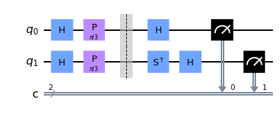
First we create the superposition state using \(H\) and \(P\) gates. We set \(\phi=\pi/3\). The goal of the quantum computation is to obtain this angle by quantum measurement. In the following quantum circuit, we use two qubits, one for \(\cos\phi\) and the other for \(\sin\phi\).

import numpy as np

from qiskit import *

# two classical registers
cr=ClassicalRegister(2,'c')

# two quantum registers (qubits)
qr=QuantumRegister(2,'q')

# set the quantum circuit
qc=QuantumCircuit(qr,cr)

# Generation of the superposition state
qc.h([0,1])
qc.p(np.pi/3,[0,1])

# separate the preparation part from the phase determination
# by placing a barrier
qc.barrier([0,1])

# real part
qc.h(0)

# imaginary part
qc.sdg(1)
qc.h(1)

# measure the both qubits
qc.measure(qr,cr)

# show the circuit
qc.draw('mpl')

# Chose a general quantum simulator without noise.
# The simulator behaves as an ideal quantum computer.
backend = Aer.get_backend('qasm_simulator')

# set number of tries
nshots=8192

# execute the quantum circuit and store the outcome
job = backend.run(qc,shots=nshots)

# extract the result
result = job.result()

# count the outcome
counts = result.get_counts()

# get the marginal counts
from qiskit.result import marginal_counts
counts_x = marginal_counts(result,indices=[0]).get_counts()
counts_y = marginal_counts(result,indices=[1]).get_counts()

# calculate the marginal probability for the sine part
q0=counts_y['0']/nshots
q1=counts_y['1']/nshots
dy=q0-q1

# calculate the marginal probability for the cosine part
p0=counts_x['0']/nshots
p1=counts_x['1']/nshots
dx=p0-p1

# evaluate the phase angle
phi=np.arctan2(dy,dx)

# print out the results
print("measured phi = {:6.3f}".format(phi))
print("exact answer = {:6.3f}".format(np.pi/3))
print("error =  {:6.3f}".format(phi - np.pi/3))

measured phi =  1.056
exact answer =  1.047
error =   0.009

The result of quantum computing is quite close to the original phase angle.

---

Last modified: 08/31/2022