Quantum computation
Contents
3.2. Quantum computation#
The construction of current quantum computers is based on the so-called quantum circuit model. It requires the following five components.
Many qubits.
The ability to reset the qubits.
A set of quantum operations (called quantum gates) that can entangle the qubits.
A classical computer that applies a circuit of quantum gates on the qubits.
The ability to measure the qubits in the computational basis and read out the classical bits.
It is necessary for you to understand the structure of the quantum computers at this stage. The very purpose of this book is to learn them. The followings are the brief summary of the construction. If you are interested in the details of the above requirements, see Ref. [1].
3.2.1. Qubits#
Quantum computers are also made of many small building blocks but unlike classical computers we need to use quantum mechanics to describe their state. Current quantum computers use the smallest quantum system, that is a two-dimensional Hilbert space \(\mathbb{C}_2\) spanned by complex vectors \(\lvert 0 \rangle\) and \(\lvert 1 \rangle\), known as qubit. These two basis states looks similar to 0 and 1 for a classical bit . However, unlike the classical bit, the state of a qubit can be in a superposition state
where \(c_0\) and \(c_1\) are complex number satisfying \(|c_0|^2+|c_1|^2=1\) (normalization). Similarly to the classical bit, we obtain either \(|0\rangle\) or \(\lvert 1 \rangle\) when the superposition state is measured. We shall call them computational basis. However, the state of the qubit is neither \(\lvert 0 \rangle\) nor \(\lvert 1 \rangle\) but \(\lvert 0 \rangle\) AND \(\lvert 1 \rangle\) simultaneously. Hence, a qubit can compute two different cases at once (if a programmer is smart enough). Quantum computers exploit this superposition state. Unlike the classical bit which has only two possible states, a qubit can take infinitely many different states since \(c_0\) and \(c_1\) can be any complex numbers satisfying the normalization condition.
Obviously, quantum computers are made of many qubits as a composite system. Let us consider two qubits, \(q_0\) and \(q_1\). A composite system of two classical bits can have four different states, ‘00’, ‘01’, 10’, and ‘11’. Similarly the pair of qubits are spanned by four basis vectors \(\lvert 00 \rangle\), \(\lvert 01 \rangle\), \(\lvert 10 \rangle\), and \(\lvert 11 \rangle\). Unlike the classical bits, the qubits can be in a superposition state
The four different possibilities are simultaneously considered in the superposition state. The complexity of the superposition state grows very rapidly as the number of qubits increases. If there are \(n\) qubits, the number of terms in the superposition state can be as many as \(2^n\). Then, \(2^n\) different cases are simultaneously computed. We will take the advantage in various applications.
In classical computers, a bit string \(b_{n-1}\, b_{n-2}\,\cdots\, b_1\, b_0\) expresses the state of the system. In quantum computer, a tensor product \(\lvert q_{n-1} \rangle \otimes \lvert q_{n-2}\rangle \otimes \cdots \otimes \lvert q_1 \rangle \otimes \lvert q_0 \rangle\) represents the state of \(n\) qubits. For two qubits, \(\lvert 01 \rangle = \lvert 0 \rangle \otimes \lvert 1 \rangle\).
3.2.2. Resetting a qubit#
Suppose that a qubit is in an arbitrary state \(|\psi\rangle\). We want to transform the state to \(|0\rangle\) or the lowest energy state. This process is known as resetting. The resetting is by no means trivial. Actually, it is very difficult due to the restrictions listed in Section 3.3 and other restrictions set by the laws of thermodynamics. The resetting on current quantum computers is not perfect.
3.2.3. Circuit models#
The time-evolution of qubits is a unitary transformation determined by the Shcrödinger equation. Quantum computers manipulate the qubits by applying a unitary operator \(U\). Starting an initial state \(|\psi_i\rangle\), the final state (the solution of the quantum computation) is mathematically given by \(|\psi_f\rangle = U |\psi_i\rangle\). The quantum algorithm determines the unitary operator \(U\). Recall that \(U\) is \(2^n \times 2^n\) matrix for \(n\) qubits, which is huge. How can we construct such a huge matrix? It turns out that a set of signle qubit unitary operators (\(2\times 2\) matrix) and two-qubit unitary operators (\(4 \times 4\)) can realize \(U\). Such unitary matrices are knwon as gates. To obtain a desired final state, we just apply a set of one-qubit gates and two-qubit gates successively. In addition to the unitaries, we also need to measure the qubits using measurement gates. The set of the gates is called quantum circuit. A simple example is given below.
3.2.4. Gates#
As a general purpose computer, a quantum computer must be able to change the state of qubits based on given instructions. Recall that a classical bit can only be flipped. In contrast, quantum computers can change the state of a qubit in infinitely many different ways. Here we use also the concept of gates. A qubit enters a gate and comes out in a different state. In other words, a state vector of the qubit is transformed to another state vector by the gate. In quantum mechanics, that is achieved by a unitary transformation \(U\). The transformation \(|\psi'\rangle=U |\psi\rangle\) in quantum mechanics is equivalent to applying a 1-qubit gate \(U\) to a qubit and expressed as
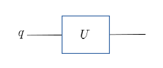
Fig. 3.4 Action of one-qubit gate.#
As an example, consider a Pauli operator \(X \equiv \sigma_x\). When it acts on the computational basis, \(X \lvert 0 \rangle = \lvert 1 \rangle\) and \(X \lvert 1 \rangle=\lvert 0 \rangle\). Hence, it acts like \(\texttt{NOT}\) in the classical computation. See the Table 3.3. The qubit can be in a superposition state. The classical truth table is not enough. When it acts on a general state, we get
which actually swaps the coefficients. The first two rows in Table 3.3 is much like the classical truth table 3.1. The third row makes quantum computers more powerful than the classical computers.
|
\(i\) |
\(o\) |
|---|---|---|
|
\(\lvert 0 \rangle\) |
\(\lvert 1 \rangle\) |
|
\(\lvert 1 \rangle\) |
\(\lvert 0 \rangle\) |
|
\(c_0 \lvert 0 \rangle + c_1 \lvert 1 \rangle\) |
\(c_1 \lvert 0 \rangle + c_0 \lvert 1 \rangle\) |
Like classical computers, quantum computers use gates that take two qubits as input. Two-qubit gates are also a unitary operator and express as
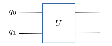
Fig. 3.5 Action of two-qubit gate.#
Logically, infinitely many 1-qubit and 2-qubits gates are possible but it is known that only several basic gates such as X, Z, and CX are actually needed to carry out quantum computation. Depending on the underlying quantum systems, the available gates are different. However, almost any gate can be expressed equivalently with a set of other gates in principle (gate decomposition). So, if a desired gate is not available on the device you are using, you must find an alternative gate.
3.2.5. Encoding#
Encoding the information of the problem to be solved to qubits in a quantum computer is not a trivial task. Let us try to use the same encoding scheme as the above classical case:
This works fine. However, there are many other encoding schemes since a qubit can take a superposition state. For example,
is another choice.
To make a good use of quantum computer, finding a good encoding scheme is crucial.
3.2.6. Circuits#
Once an encoding scheme is chosen, we need to give a set of instructions to a quantum computer. That is we find a set of unitary operators that are applied on qubits one after the other. Unlike classical computation, no advanced programming language is available for quantum computing. Therefore, programmers must right instructions the device can understand directly (similar to coding with machine or assembly language for classical computers.) A code for quantum computation looks like

Fig. 3.6 An example of quantum circuit.#
which is known as quantum circuit. Each object in the circuit is a unitary gate.
The following circuit computes \(x \oplus y\) using a quantum computer.
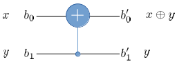
Fig. 3.7 Quantum computation of \(x \oplus y\).#
The gate in the circuit is known as controlled X or controlled NOT. It applies \(X\) on \(q_0\) only when \(q_1 = \lvert 1 \rangle\). This is equivalent to the classical computation with \(\texttt{XOR}\) gate if input qubits are either \(\lvert 0 \rangle\) or \(\lvert 1 \rangle\). We can see the difference between classical and quantum computation when a superposition state is used as input. Consider a case where \(q_0=\lvert 0 \rangle\) and \(q_1=c_0 |0 \rangle + c_1 \lvert 1 \rangle\). The state of the two qubits is
The output is
which is known as entangled state. There is no way to express this state in a classical computer. Quantum computation utilizes entangled states.
3.2.7. Readouts#
When a qubit is in \(\lvert 0 \rangle\) or \(\lvert 1 \rangle\), readout is in principle accurate (not on current NISQ computers due to device errors). However, the outcome is completely uncertain if the qubit is in a superposition state (3.1). We will obtain \(\texttt{0}\) or \(\texttt{1}\) at random. If we prepare many qubits in the same superposition state, we obtain \(\texttt{0}\) from some and \(\texttt{1}\) from others. Hence, the readout of qubits is stochastic, from which we know that the qubits are in a superposition state but which one? The principle of quantum mechanics tells us that the probability of getting \(\texttt{0}\) is given by \(|c_0|^2\) and \(\texttt{1}\) by \(|c_1|^2\). By measuring many qubits in the same state, we can calculate the probabilities from which \(|c_0|^2\) and \(|c_1|^2\) can be determined. The phase of \(c_0\) and \(c_1\) are still missing. There is a complicate procedure, known as quantum tomography, which can determine the superposition state if and only if sufficiently large number of the same superposition states are measured. Therefore, it is necessary to repeat the same quantum computation many times if the final result is a superposition state. Even when the result of the computation is designed to be \(\lvert 0 \rangle\) or \(\lvert 1 \rangle\) by the algorithm, the outcome can be a superposition state due to device errors. Even worse, the final state can be so-called mixed state, which contains a mixture of classical and quantum uncertainties simultaneously. A good quantum circuit avoids both classical and quantum uncertainties as much as possible.
Last modified on 08/30/2022.