6.2. More qubits

Two qubits are too few for useful quantum computation and we need many more. In this section, we consider \(n\) qubits where \(n>2\). Each qubit is in \(\mathbb{C}^2\) and thus ther system of \(n\) qubits is in \(2^n\) dimensional Hilbert space \(\mathbb{C}^2 \otimes \cdots \otimes \mathbb{C}^2\), which spanned by \(2^n\) basis vectors.

6.2.1. Notation

In this book, we write the computational basis of \(n\) qubits as

\[ |q_{n-1}\, q_{n-2}\, \cdots\, q_1\, q_0\rangle \equiv |q_{n-1}\rangle \otimes |q_{n-2}\rangle \otimes \cdots \otimes |q_1\rangle \otimes |q_0\rangle \]

Notice that the qubits are ordered from the right to the left. For example, \(|01011\rangle\) is a computational basis ket for five qubits representing \(|0\rangle \otimes |1\rangle \otimes |0 \rangle \otimes |1\rangle \otimes |1\rangle\).

For large \(n\), the expression becomes very long. We use a shorthand expression or an index based on integers in classical binary strings:

\[ |j\rangle_n = |j_{n-1}\, j_{n-2}\, \cdots\, j_1\, j_0\rangle \]

where \(j_k \in \{0,1\}\) and

\[ j = 2^{n-1} j_{n-1} + 2^{n-2} j_{n-2} + \cdots + 2 j_1 + j_0 = \sum_{k=0}^{n-1} 2^k j_k. \]

For \(n=3\), we have eight basis vectors

\[\begin{split} \begin{align} &|0\rangle_3 = |000\rangle, && |1\rangle_3 = |001\rangle, &&& |2\rangle_3 = |010\rangle, &&&&|3\rangle_3 = |011\rangle\\ &|4\rangle_3 = |100\rangle, && |5\rangle_3 = |101\rangle, &&& |6\rangle_3 = |110\rangle, &&&&|7\rangle_3 = |111\rangle \end{align} \end{split}\]

---

Exercise For the system of 5 qubits, find what computational basis set \(|13\rangle_5\) means.

6.2.2. Entanglement

Recall the system is entangled if the state vector of a composite system cannot be written as a product of individual state vectors. For two qubits, this definition is clear. For three qubits, what does “product” state mean? Do all three qubits have to be separated like \(|q_2\rangle \otimes |q_1\rangle \otimes |q_0\rangle\)? If \(q_1\) and \(q_2\) are entangled but not with \(q_0\) the state vector can be written as

\[ |\text{entangled}\rangle_2 \otimes |q_0\rangle \]

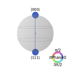
Is this a product state? In one sense this is a product state and thus the whole system is not entangled. However, a part of the whole system is entangled. When the state vector of a whole system cannot be written as any form of product state, we say that the whole system is entangled. For example, the state known as the GHZ state:

\[ |\text{GHZ}\rangle = \frac{1}{\sqrt{2}}\left(|000\rangle + |111\rangle\right) \]

cannot be written as any form of product state. We say that the state is maximally entangled. To understand the effect of entanglement, qubits \(q_0\), \(q_1\) and \(q_2\) are delivered to Alice, Bob, and Charlie, respectively. Before any measurement, all of them have a equal chance to get \(|0\rangle\) or \(|1\rangle\). Alice measures her qubit before others and get \(|1\rangle\). Immediately, the state collapse to \(|111\rangle\) and she knows that Bob’s and Charlie’s qubits are both in \(|1\rangle\). Now, they have no chance to get \(|0\rangle\) (but they don’t know it.) This happens even when they are far apart. In one sense, this entanglement is strong because measurement of a single qubit removes the uncertainty in two others. On the other hand, the entanglement is not robust since the measurement of a single qubit destroys the entanglement entirely. The GHZ state is used in various quantum algorithms including Quantum Byzantine agreement.

There is another maximally entangled state known as the W state

\[ |\text{W}\rangle = \frac{1}{\sqrt{3}} \left(|001\rangle + |010\rangle + |100\rangle\right). \]

Again, Alice measures her qubit first but gets \(|0\rangle\) this time. The state collapses to \(\frac{1}{\sqrt{2}}\left(01\rangle + |10\rangle\right) \otimes |0\rangle\). This entanglement is a little bit more robust than the GHZ state since even after Alice measured, entanglement between Bob and Charie remains.

Finding all maximally entangled states for bigger composite systems is not a trivial task. We will not discuss it here.

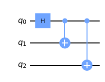
Quiskit example: creation of GHZ state

The GHZ state can be created essentially in the same way as the Bell state \(|\Phi^{+}\rangle\). The following circuit creates it using H and CX gates.

from qiskit import *

qr=QuantumRegister(3,'q')
qc=QuantumCircuit(qr)

qc.h(0)
qc.cx(0,1)
qc.cx(0,2)

qc.draw('mpl')

from qiskit.quantum_info import Statevector

psi=Statevector(qc)
psi.draw('latex')

\[\frac{\sqrt{2}}{2} |000\rangle+\frac{\sqrt{2}}{2} |111\rangle\]

from qiskit.visualization import plot_state_qsphere
# it's an entangled state.  Use qsphere.
plot_state_qsphere(psi,figsize=(4,4))

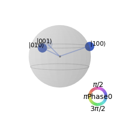
Generating W state is a little bit more complicated. The following circuit creates the W state.

from qiskit import *
import numpy  as np

qr=QuantumRegister(3,'q')
qc=QuantumCircuit(qr)

theta = 2*np.arccos(1./np.sqrt(3))

qc.ry(theta,0)
qc.ch(0,1)
qc.cx(1,2)
qc.cx(0,1)
qc.x(0)

qc.draw('mpl')

from qiskit.quantum_info import Statevector

psi=Statevector(qc)
psi.draw('latex')

\[\frac{\sqrt{3}}{3} |001\rangle+\frac{\sqrt{3}}{3} |010\rangle+\frac{\sqrt{3}}{3} |100\rangle\]

plot_state_qsphere(psi,figsize=(4,4))