8.5. A little example of quantum parallelism

8.5.1. The Objective

Quantum computer can calculate many different instances simultaneously. Here we consider a simple example. Suppose that we want to calculate \(z = x \oplus y\) where \(x,\, y,\, z \in \{0,1\}\). The variables are assigned to three qubits as \(|zyx\rangle = |z\rangle \otimes |y\rangle \otimes |x\rangle\). Initially, \(z=0\). The computation corresponds to transformation \(|0\rangle \otimes |y\rangle \otimes |x\rangle \Rightarrow |x \oplus y\rangle \otimes |y\rangle \otimes |x\rangle\). There are four possible instances:

\[\begin{split} \begin{align} |000\rangle \quad &\Rightarrow \quad |000\rangle \\ |001\rangle \quad &\Rightarrow \quad |101\rangle \\ |010\rangle \quad &\Rightarrow \quad |110\rangle \\ |011\rangle \quad &\Rightarrow \quad |011\rangle \end{align} \end{split}\]

We want to compute all these four cases at once.

8.5.2. Algorithm

We use a superposition state of the four input states. First we create four possible input states with equal weight and then we compute \(x\oplus y\) for each term:

\[\begin{split} \begin{align} |000\rangle &\Rightarrow |0\rangle \otimes \frac{1}{2}\left(|0\rangle\otimes|0\rangle+|0\rangle\otimes|1\rangle+|1\rangle\otimes|0\rangle + |1\rangle\otimes|1\rangle \right) \\ &\Rightarrow \frac{1}{2}\left(|000\rangle + |101\rangle + |110\rangle + |011\rangle \right) \end{align} \end{split}\]

Note that the output does not include all possible states. For example \(|111\rangle\) does not exist since \(1\oplus 1 \ne 1\).

The first step can be done with the Walsh-Hadamard transformation. The addition can be done with thee CX gates as shown in Section 8.4. The following Qiskit example evaluates the four cases simultaneously.

8.5.3. Qiskit Example

Circuit

from qiskit import *

cr=ClassicalRegister(3,'c')
qr=QuantumRegister(3,'q')
qc=QuantumCircuit(qr,cr)

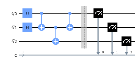
qc.h([0,1])
qc.cx(0,1)
qc.cx(1,2)
qc.cx(0,1)
qc.barrier()
qc.measure(qr,cr)
qc.draw('mpl')

Execution (noiseless)

# Chose a general quantum simulator without noise.
# The simulator behaves as an ideal quantum computer.
backend = Aer.get_backend('qasm_simulator')

# set number of tries
nshots=8192

# execute the quantum circuit and store the outcome
job = backend.run(qc,shots=nshots)

# extract the result
result = job.result()

# count the outcome
counts = result.get_counts()

from qiskit.visualization import plot_histogram
plot_histogram(counts)

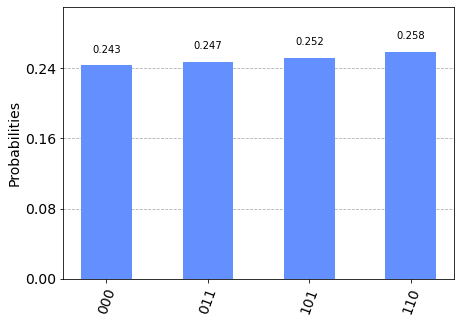
Only four states are obtained and each shows \(z = x \oplus y\). We indeed calculated four different cases at once thanks to the quantum parallelism.

Execution (noisy)

# simulating IBL Jakarta device
from qiskit.providers.fake_provider import FakeJakarta

backend = FakeJakarta()

# set the number of tries
nshots=8192

# execute the circuit
job = backend.run(qc,shots=nshots)

# extract the result
result = job.result()

# count the outcome
counts = result.get_counts()

from qiskit.visualization import plot_histogram
plot_histogram(counts)

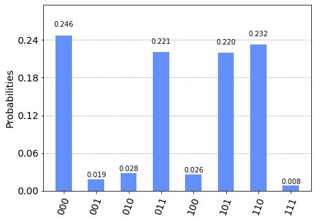
Notice that additional states appeared due to the noises. However, their probabilities are small and we can easily identify the four major peaks.

---

Last modified: 08/31/2022