Quantum Phase Estimation
Contents
8.8. Quantum Phase Estimation#
The problem of quantum phase estimation (QPE) is just a special kind of eigenvalue problem. However, it plays a quite important role in quantum computation. It can be considered as a subroutine used in many useful quantum algorithms such as factorization, quantum walks, … So, we need to learn it before other quantum algorithms.
8.8.1. The problem#
Consider a unitary operator \(U\) in a \(2n\)-dimension Hilbert space \((\mathbb{C}_2)^{\otimes n}\). Its eigenvector \(|psi_\lambda\rangle\) satisfies the eigenvalue equation \(U |\psi_\lambda\rangle = \lambda |\psi_\lambda\rangle\) where \(\lambda\) is the eigenvalue. The adjoint of the eigenvalue equation is \(\langle \psi_\lambda| U^\dagger = \langle \psi_\lambda| \lambda^*\). The inner product of the two eigenvalue equations is \(\langle \psi_\lambda| U^\dagger U |\psi_\lambda\rangle = |\lambda|^2 \langle\psi_\lambda|\psi_\lambda\rangle\). Since \(U\) is unitary, \(U\dagger U = I\) and thus \(|\lambda|=1\). So, the eigenvalue equation can be written as
where \(|\psi_\theta\rangle\) is the eigenvector and the corresponding eigenvalue is \(e^{2\pi i\theta}\). Our task is to find the phase variable \(\theta \in [0,1)\) for a given \(|\psi_\theta\). Mathematically, it is a trivial problem. Assuming \(|\psi_\theta\rangle\) is normalized, \(e^{2\pi i \theta} = \langle \psi_\theta | U | \psi_\theta \rangle\), which current quantum computer cannot compute. Can we find \(\theta\) without computing the inner product?
8.8.2. Encoding a continuous number between 0 and 1#
The value we want to find is not integer. How can we encode a continuous number between 0 and 1 in qubits? Since it is not possible to encode a true continuous number in digital computers, we approximate it. In Section 8.4 we encoded integers between \(0\) and \(2^n-1\) in \(n\) qubits as \(|j\rangle_n = |j_{n-1}\,j_{n-2}\,\cdots\,j_{0} \rangle\). Noting that \( 0 \le 2^n \theta < 2^n\), we can encode \(2^n \theta\) as an integer state \(|j\rangle_n\). Then, \(\theta = j/2^n\), which is not continuous and there is a gap of \(2^{-n}\). The gap decreases quickly as \(n\) increases. If an accurate value of \(\theta\) is needed, we must use a large number of qubits.
Our task is now to find the integer state \(|j\rangle_n\) corresponding to \(\theta\).
8.9. #
8.9.1. The algorithm#
The QPE algorithm was developed by Kitaev in 1995 [9].
We use \(n+1\) qubits. The first \(n\) qubits are used to from the computational basis \(\ell\rangle_n\, \ell=0,\cdots, n-1\) and \(the remaining qubit stores \)|psi\rangle$. The first step of our strategy is to create the following state:
We try to find a quantum algorithm that transforms it to \(|j\rangle_n \otimes |\psi\rangle\). In other words, the algorithm eliminates the integer states expect for \(|j\rangle_n\). Since there is one term at the end, measurement detects \(|j\rangle_n\) with high certainty.
We can generate (8.18) using the Walsh-Hadamard transformation discussed in Section 8.4. Furthermore, we know that Eq. (8.18) is equivalent to
Next we consider a controlled gate \(CU^{2^i}\) which applys the unitary operator \(U\) \(2^i\) times on \(\psi\rangle\) when \(i\)-th qubit is in \(1\rangle\) and does nothing otherwise. For example, the \(i\)-th qubit is transformed as (only the \(i\)-qubit and \(|psi\rangle\) are shown)
Applying the gate to all qubits (except for \(|\psi\rangle\)),
Recall that \(2^n \theta\) is an integer as discussed in Section 8.8.2. Hence, we have Fourier transform of a computational basis.
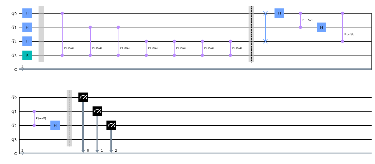
The final step is to apply inverse Fourier transform.
We have obtained a desired state. Suppose that we obtain \(|j\rangle\) up on the measurement with high probability, then \(\theta = j/2^n\).
If the number of qubits is not big enough, \(2^n \theta\) can deviate from any integer. Nevertheless, the chance to find the nearest integer \(j\) is much high than other integers. Thence, this algorithm gives us a good estimate of \(\theta\). See the discussion of the error in [10].
8.9.2. Example#
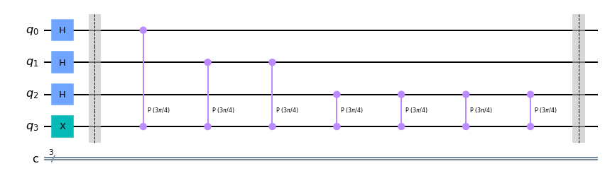
Consider a unitary operator \(U = T^3\). \(|1\rangle\) is known to be its eigenket. We want to find the phase of angle \(\theta\) of the corresponding eigenvalue. Since the value of \(\theta\) is not known, we don’t know how many qubits are needed. Let us try three qubits for the expression of \(\theta\) and another qubit for \(|psi\rangle\). We need also three classical bits for measurement. \(T^3\) can be realized by the pase gate \(P(3\pi/4)\).
import numpy as np
from qiskit import *

cr=ClassicalRegister(3,'c')
qr=QuantumRegister(4,'q')
qc=QuantumCircuit(qr,cr)

# Walsh-Hadamard transformation for qubit 0-2
qc.h(range(3))

# X for qubit 3 to create |1>
qc.x(3)

qc.barrier()

# qubit 0
qc.cp(np.pi*3/4,0,3)

# qubit 1
qc.cp(np.pi*3/4,1,3)
qc.cp(np.pi*3/4,1,3)

# qubit 2
qc.cp(np.pi*3/4,2,3)
qc.cp(np.pi*3/4,2,3)
qc.cp(np.pi*3/4,2,3)
qc.cp(np.pi*3/4,2,3)

qc.barrier()

qc.draw('mpl')
# Inverse Fourier transform

# SWAP
qc.swap(0,2)

# qubit 0
qc.h(0)

# qubit 1
qc.cp(-np.pi/2,1,0)
qc.h(1)

# qubit 2
qc.cp(-np.pi/4,2,0)
qc.cp(-np.pi/2,2,1)
qc.h(2)

qc.barrier()

qc.measure(0,0)
qc.measure(1,1)
qc.measure(2,2)

qc.draw('mpl')
# Chose a general quantum simulator without noise.
# The simulator behaves as an ideal quantum computer.
backend = Aer.get_backend('qasm_simulator')

# set number of tries
nshots=8192

# execute the quantum circuit and store the outcome
job = backend.run(qc,shots=nshots)

# extract the result
result = job.result()

# count the outcome
counts = result.get_counts()

from qiskit.visualization import plot_histogram
plot_histogram(counts)
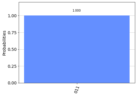
We obtain \(|011\rangle = |3\rangle_3\) with unit probability. The quantum algorithm has selected \(j=3\) out of 8 integers. Hence, \(\theta = 3 / 2^3 = 3/8\). The result is in perfect agreement with the actual eigenvalue \(e^{i \pi 3/4} = e^{2\pi i 3/8}\).
What will happen if we use more qubits than necessary? Let us try 4 qubits. There are 16 integer numbers to chose. If \(j=6\) is selected, we should get the same answer. The following code indeed finds 6 as the answer.
import numpy as np
from qiskit import *

cr=ClassicalRegister(4,'c')
qr=QuantumRegister(5,'q')
qc=QuantumCircuit(qr,cr)

# Walsh-Hadamard transformation for qubit 0-2
qc.h(range(4))

# X for qubit 3 to create |1>
qc.x(4)

qc.barrier()

for i in range(4):

# qubit 0
    for _ in range(2**i):
        qc.cp(np.pi*3/4,i,4)

qc.barrier()

# SWAP
qc.swap(0,3)
qc.swap(1,2)

# qubit 0
qc.h(0)

# qubit 1
qc.cp(-np.pi/2,1,0)
qc.h(1)

# qubit 2
qc.cp(-np.pi/4,2,0)
qc.cp(-np.pi/2,2,1)
qc.h(2)

# qubit 3
qc.cp(-np.pi/8,3,0)
qc.cp(-np.pi/4,3,1)
qc.cp(-np.pi/2,3,2)
qc.h(3)

qc.barrier()

qc.measure(0,0)
qc.measure(1,1)
qc.measure(2,2)
qc.measure(3,3)

# Chose a general quantum simulator without noise.
# The simulator behaves as an ideal quantum computer.
backend = Aer.get_backend('qasm_simulator')

# set number of tries
nshots=8192

# execute the quantum circuit and store the outcome
job = backend.run(qc,shots=nshots)

# extract the result
result = job.result()

# count the outcome
counts = result.get_counts()

from qiskit.visualization import plot_histogram
plot_histogram(counts)
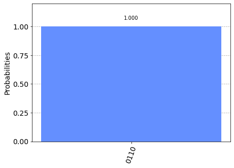
Now we got \(|0110\rangle = |6\rangle\) from which we find \(\theta = 6/2^4 = 3/8\). The result does not change.
8.9.3. Irrational value#
If the eigenvalue is \(e^{2\pi i /3}\), \(theta=1/3\) cannot be expressed by the finite binary fractions and thus it is not possible to get the perfect answer using the current algorithm. Let us consider \(U=P(2\pi/3)\) and \(\psi\rangle=|1\rangle\).
import numpy as np
from qiskit import *

cr=ClassicalRegister(4,'c')
qr=QuantumRegister(5,'q')
qc=QuantumCircuit(qr,cr)

# Walsh-Hadamard transformation for qubit 0-2
qc.h(range(4))

# X for qubit 3 to create |1>
qc.x(4)

qc.barrier()

for i in range(4):

# qubit 0
    for _ in range(2**i):
        qc.cp(np.pi*2/3,i,4)

qc.barrier()

# SWAP
qc.swap(0,3)
qc.swap(1,2)

# qubit 0
qc.h(0)

# qubit 1
qc.cp(-np.pi/2,1,0)
qc.h(1)

# qubit 2
qc.cp(-np.pi/4,2,0)
qc.cp(-np.pi/2,2,1)
qc.h(2)

# qubit 3
qc.cp(-np.pi/8,3,0)
qc.cp(-np.pi/4,3,1)
qc.cp(-np.pi/2,3,2)
qc.h(3)

qc.barrier()

qc.measure(0,0)
qc.measure(1,1)
qc.measure(2,2)
qc.measure(3,3)

# Chose a general quantum simulator without noise.
# The simulator behaves as an ideal quantum computer.
backend = Aer.get_backend('qasm_simulator')

# set number of tries
nshots=8192

# execute the quantum circuit and store the outcome
job = backend.run(qc,shots=nshots)

# extract the result
result = job.result()

# count the outcome
counts = result.get_counts()

from qiskit.visualization import plot_histogram
plot_histogram(counts)
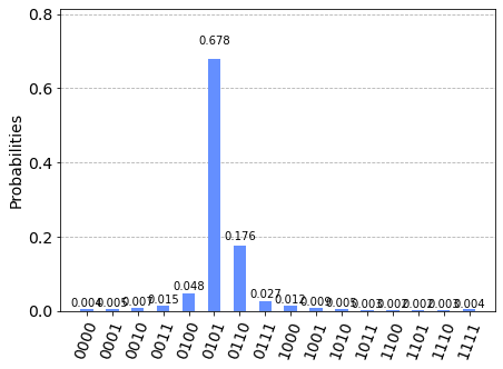
Clearly \(|0101\rangle = |5\rangle\) is dominant. It corresponds to \(\theta = 5/2^4 = 0.3125\). The exact answer is \(1/3=0.3333...\). The agreement is not bad and the error can be reduced by using more qubits.
Last modified on 07/24/2022.