
4. Root Finding#
In this chapter, we try to find real roots of a function \(f(x)\), that is to solve \(f(x)=0\). Finding roots of a function is a ubiquitous mathematical procedure in physics. For example, an equilibrium position of a particle in a potential field is determined as the place where the force is zero, i.e., \(U'(x)=0\). In many cases, the equation is transcendental and no analytical solution is available. Even when an analytical solution is known, numerical evaluating it may suffer from the round-off error as discussed in Sec Section 1.7.1. In this chapter, we discuss how to find a root of a given equation \(f(x)\) within acceptable error \(\epsilon\) (tolerance). There are a variety of methods but almost all of them use an iterative method. It starts with an candidate of the root and check if it is good enough. If not, a new candidate is proposed. Then, the process is repeated until a reasonable root is found. The iterative method requires three steps.
Proposing a reasonable initial candidate This is not a trivial step. It will be useful if we a rough idea where is the root you ware looking for. For example, if we know that the root is somewhere between \(x_L\) and \(x_U\), it is much easier to find it. The process to find the lower bound \(x_L\) and the upper bound \(x_U\) is called bracketing the root. The easiest way to bracket the root is to plot \(f(x)\) and to visually find the bracket by direct inspection.
Proposing a new candidate There are many methods. All of them use the information of previous candidates. For example, some use the derivative of \(f(x)\) at the previous candidate to predict the root. Other use several previous candidates and to predict a new one. As the iteration continues, we gain more information about the function and are able to find a better candidate.
Termination of the iteration We cannot repeat the iteration forever and there must be rule to terminate it. We want to stop the iteration when the difference between the candidate and the root is small enough. However, such error cannot be obtained unless we know the exact root. Hence, we are only able to make an estimate of the error. There are several methods to do so.
The standard methods have some limitation. If a root is well separated from others (Fig. Fig. 4.1A), it is relatively easy to find it. If two roots are very close to each other (Fig. Fig. 4.1B), it is difficult find them. When two roots are degenerate (Fig. Fig. 4.1C), the standard methods are powerless. In this lecture, we do not attempt to solve the latter two cases.
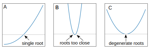
Fig. 4.1 (A) It is rather easy to find an isolated root. (B) When two roots are close together, it is diffcult to find them. (C) When two roots are degenerate, the standard methods fail to find them.#
There are other cases the standard root-finding method fail. For example. consider \(\sqrt{x-a} = 0\). The root is \(x=a\). Note that the function is not defined for \(x < a\). If a proposed candidate \(x_n\) is below \(a\) where the function is undefined, the iteration cannot continue. This happens when the function has the finite support and the root is located at the boundary of the support. In most cases, you can see the root at the boundary by direct inspection and a numerical method is not needed.
Last modified on 3/11/2024 by R. Kawai.