2.3.1. An Overdamped Motion

A classical particle of mass \(m\) is in a periodic potential field \(U(x) = U_0 \cos(2\pi x/\lambda)\) where \(U_0 > 0\) is a strength of the potential and \(\lambda > 0\) is the wave length. The space is filled with a viscous fluid and thus a strong friction force acts on the particle when it moves. Its motion is determined by the Newton’s equation of motion:

\[ m \ddot{x} = - \gamma \dot{x} + \frac{2\pi U_0}{\lambda} \sin\left(\frac{2\pi x}{\lambda}\right) \]

where \(\gamma>0\) is the friction constant. The friction is so strong that the inertial term \(m \ddot{x}\) can be neglected (overdupmed). Using the normalized coordinate \(\xi =\displaystyle\frac{2\pi x}{\lambda}\) and time \(\tau = \displaystyle\frac{U_0}{\gamma} \left(\displaystyle\frac{2\pi}{\lambda}\right)^2 t\), the equation of motion becomes

\[ \frac{d}{d\tau} \xi = \sin(\xi) \]

The solution to this differential equation is given by [5]

\[ \tau = \ln \left|\frac{\csc \xi_0+\cot \xi_0}{\csc \xi + \cot \xi} \right| \]

where \(\xi_0\) is the initial position. While this is exact, it is very difficult to interpret. We want to know the position of the particle as a function of time, that is \(\xi(\tau)\). Instead we have \(\tau(\xi)\). It seems impossible to invert the above expression. So, we resort to a numerical method. Inverting a function on the graph is simple. Just swap the vertical and the horizontal axes. We calculate \(\tau(\xi)\) and plot the curve with the horizontal axis as \(\tau\) and the vertical axis as \(\xi\). To do so, we need to know the range of \(\xi\). What we are sure is that the particle moves toward the nearest potential minimum and it does not move once it reaches the minimum, which is \((2n+1)\pi\) where \(n\) is an integer. So, the range of \(\xi\) is \([\xi_0, (2n+1) \pi]\) if \(2\pi n < \xi_0 < (2n+1)\pi\) and \([(2n-1)\pi, \xi_0]\) if \((2n-1)\pi < \xi_0 < 2n \pi\).

import numpy as np
import matplotlib.pyplot as plt

def f(x,x0):

    y = np.log((1/np.sin(x0)+1/np.tan(x0))/(1/np.sin(x)+1/np.tan(x)))
    return y
    
# chose the initial position between 0 and pi/2
x0 = 0.1

# the nearest potential minimum
x1 = np.pi

# the grid point between x0 and x1
# the final point is slightly before the minimum
x = np.linspace(x0,x1-1e-5,101)

t = f(x,x0)

plt.plot(t,x,'-k')
plt.axhline(y = x1, color = '0.8', linestyle = '--') 
plt.ylim([x0-0.5,x1+0.5])
plt.xlabel(r"$\tau$")
plt.ylabel(r"$\xi(\tau)$")
plt.text(0,x1+0.1,r"$\xi=\pi$ (potential minimum)")
plt.show()

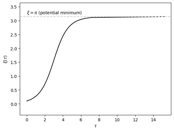
The plot indicates that the particle initially accelerates toward the destination but slows down after \(\xi=\pi/2\). By \(\tau=7\), the particle is almost at the minimum. After that the particle moves very slowly and seems never reach the minimum. Mathematically, it can be shown that the the particle approaches the minimum asymptotically and never arrives the exact minimum. [5]

---

Last modified on 3/10/2024 by R. Kawai.