1.7. Applications

1.7.1. Roots of quadratic equations

Many physics applications such as molecular dynamics simulation need to solve quadratic equations: \(a x^2 + b x + c = 0\). Its solitions are well known. If \(a\ne 0\), we have the standard formula:

(1.1)\[ x_+ = \frac{-b + \sqrt{b^2 - 4 a c}}{2 a}, \qquad x_- = \frac{-b - \sqrt{b^2 - 4 a c}}{2 a} \]

When \(a=0\), we have only one solution \(x_0=-c/b\). There seems no problem evaluating these solutions. However, in some cases, computers give us wrong answers.

The coefficients, \(a\), \(b\), and \(c\) change as the computation proceeds. Think what will happen to the two solution when \(a\) becomes very small. One solution should be close to \(x_0\). How about the other? A bad thing happens to the other solution. To seee that, let assume \(a>0\) and \(b>0\) for moment. Take a look at the numerator of \(x_+\). \(\sqrt{b-4ac}\) is only slightly smaller than \(b\). Recall that computers are not good at evaluating the difference between two similar values.

Fortunately, there is a simple way to avoid the loss of significant figures:

\[ x_+ = \frac{-b + \sqrt{b^2 - 4 a c}}{2 a} = \frac{2c}{-b+\sqrt{b^2 - 4 a c}} = \frac{c}{a x_-} \]

which does not involve the severe substraction.

Algorithm 1.6.1 Roots of quadratic equations Roots of \(a x^2 + b x + c = 0\) (\(a\ne 0\) and \(b\ne 0\)) are given by

(1.2)\[\begin{split} \begin{eqnarray} x_1 &=& \frac{-b - \text{sign}(b)\sqrt{b^2 - 4 a c}}{2a} \\ x_2 &=& \frac{c}{a x_1} \end{eqnarray} \end{split}\]

where the signum function \(\text{sign}(x)\) is defined by

\[\begin{split} \text{sign}(x) = \begin{cases} +1 & x>0 \\ -1 & x<0 \end{cases} \end{split}\]

import numpy as np
import matplotlib.pyplot as plt

b=1.0
c=0.25
a=1.0
x=np.zeros(50)
y1=np.zeros(50)
y2=np.zeros(50)
n=0
while a > np.finfo(float).eps:
    x[n]=a
    d=b**2-4*a*c
    y1[n]=(-b+np.sqrt(d))/(2.0*a)
    y2[n]=-2*c/(b+np.sqrt(d))
    print("a={0:8.2e}, regular={1:22.16e}, smart={2:22.16e}"
          .format(x[n],y1[n],y2[n]))
    n+=1
    a=a/10.

plt.ioff()
plt.figure(figsize=(6,5))
plt.loglog(x[0:n],abs(y2[0:n]+0.25), 'ob', label='smart')
plt.loglog(x[0:n],abs(y1[0:n]+0.25), 'or', label='regular')
plt.legend(loc=4)
plt.xlabel('a')
plt.ylabel('$|x-x_0|$')
plt.show()

a=1.00e+00, regular=-5.0000000000000000e-01, smart=-5.0000000000000000e-01
a=1.00e-01, regular=-2.5658350974743116e-01, smart=-2.5658350974743099e-01
a=1.00e-02, regular=-2.5062814466900174e-01, smart=-2.5062814466900230e-01
a=1.00e-03, regular=-2.5006253126952371e-01, smart=-2.5006253126954492e-01
a=1.00e-04, regular=-2.5000625031246226e-01, smart=-2.5000625031251955e-01
a=1.00e-05, regular=-2.5000062500168951e-01, smart=-2.5000062500312503e-01
a=1.00e-06, regular=-2.5000006248498957e-01, smart=-2.5000006250003121e-01
a=1.00e-07, regular=-2.5000000625219337e-01, smart=-2.5000000625000030e-01
a=1.00e-08, regular=-2.5000000403174732e-01, smart=-2.5000000062500000e-01
a=1.00e-09, regular=-2.5000002068509269e-01, smart=-2.5000000006250001e-01
a=1.00e-10, regular=-2.5000002068509269e-01, smart=-2.5000000000625000e-01
a=1.00e-11, regular=-2.5000002068509269e-01, smart=-2.5000000000062500e-01
a=1.00e-12, regular=-2.5002222514558520e-01, smart=-2.5000000000006251e-01
a=1.00e-13, regular=-2.5035529205297274e-01, smart=-2.5000000000000627e-01
a=1.00e-14, regular=-2.4980018054066019e-01, smart=-2.5000000000000061e-01
a=1.00e-15, regular=-2.7755575615628914e-01, smart=-2.5000000000000006e-01

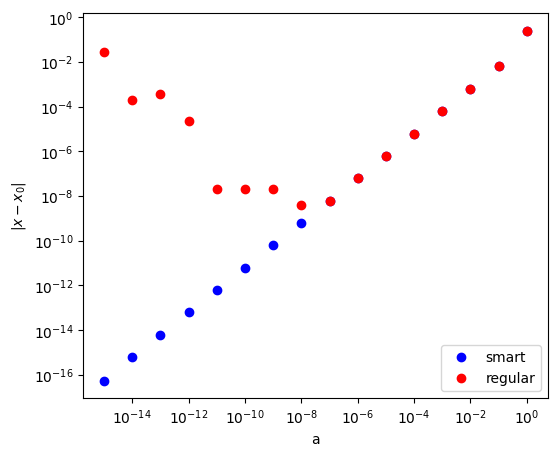
The result of smart formular Eq. (1.2) approaches the correct limit as \(a \rightarrow 0\). On the other hand, standard formular (1.1) becomes errorneous for \(a<10^{-7}\). In fact, a graduate student who was investing non-equilibrium thermal processes using hard disc molecular dynamics suffered from this error.

---

Last modified on 2/12/2024 by R. Kawai.