3.3. Second order derivative

3.3.1. Three-point method

We can evaluated the second order derivative using the mean value method twice. First, we pretend that the first order derivative is known. Using the mean value method with step size \(h/2\), we obtain

\[ f''(x) \approx \Delta_M f'(x) = \frac{f'(x+\frac{h}{2})-f'(x-\frac{h}{2})}{h} \]

Then, we replace the first order derivatives with approximated ones using the mean value method again.

\[\begin{split} \begin{eqnarray} f'(x+\frac{h}{2}) &\rightarrow& \Delta_M f(x+\frac{h}{2}) = \frac{f(x+h)-f(x)}{h} \\ f'(x-\frac{h}{2}) &\rightarrow& \Delta_M f(x-\frac{h}{2}) = \frac{f(x)-f(x-h)}{h}. \end{eqnarray} \end{split}\]

The result is

(3.3)\[ f''(x) \approx \Delta^{(2)}_M f(x) \equiv \displaystyle\frac{f(x+h)+f(x-h)-2f(x)}{h^2}. \]

where \(\Delta^{(2)}_M\) is the second order mean finite difference operator. Using the Taylor expansion, we find that the error of this approximation is the order of \(h^2\), the same as the first order mean value method.

Method 2.3.1: Three-point finite difference method of the second order derivative

\[ \frac{d^2f}{dx^2} = \frac{f(x+h)+f(x-h)-2f(x)}{h^2} + \mathcal{O}(h^2) \]

Example 2.3.1

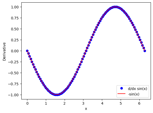
The second order derivative of \(\sin(x)\) is \(-\sin(x)\). let us evaluate the second order derivative of \(\sin(x)\) at \(x=2 n \pi / N\) where \(n=0, 1, \cdots, N\). Use \(N=100\) and plot the result. Verify that it is \(-\sin(x)\) at least within the accuracy of the numerical method.

import numpy as np

h=0.01
N=100

# define the evaluation points
x=np.linspace(0,2*np.pi,N+1)

# f(x)
fc=np.sin(x)

# f(x+h)
ff=np.sin(x+h)

# f(x-h)
fb=np.sin(x-h)

# second order derivative
df=(ff+fb-2*fc)/h**2

# plot derivative d/dx sin(x) as circle and -sin(x) as red line
import matplotlib.pyplot as plt

plt.xlabel('x')
plt.ylabel('Derivative')
plt.plot(x,df, 'ob', label='d/dx sin(x)')
plt.plot(x,-fc,'-r', label='-sin(x)')
plt.legend(loc=4)

<matplotlib.legend.Legend at 0x7f5304306920>

3.3.2. Five-point method

Better accuracy can be obtained by the five-point method.[10] Its error is the order of \(h^4\).

Method 2.3.2: Five-point finite difference method for 2nd order derivative

\[ \frac{df}{dx} = \frac{-f(x+2h) + 16 f(x+h) - 30 f(x) + 16 f(x-h) -f(x-2h)}{12h^2} + \mathcal{O}(h^4) \]